
 Email Alerts
 RSS
RSS
Numerical simulation of internal wave propagation in two-layer fluid under two water surface boundary conditions
-
摘要: 基于FLUENT计算流体力学软件及其二次开发功能,采用VOF(Volume of Fluid)多相流模型,在
$k{\text{-}}\varepsilon$ 湍流模型下建立了模拟内波传播的分层数值水槽。设置两层稳定分层,以上下层不同密度差和水深比设置工况,利用平板拍击法造波。在刚盖和自由表面两种上边界条件下进行数值模拟并与各自的理论解进行比较,分析了两者之间的异同。研究发现密度差的改变不会明显影响理论解与数值解之间的一致程度;上下两层流体深度差值的改变会明显影响数值计算结果。上层水深很小时,在自由表面假定下水气交界面处出现了较为明显的垂向速度;在两种假定下,数值模拟的水平速度都体现了非线性的影响。而当下层水深很小时,非线性的影响微弱。鉴于在实际海洋中上层水深远小于下层水深,尤其是当计算运动幅值更大的内孤立波时,采用更为真实的自由表面假定更为合理。Abstract: Based on the FLUENT computational fluid dynamics software and its secondary development function, as well as the VOF (Volume of Fluid) multiphase flow model, a stratified numerical water flume that simulates the propagation of oceanic internal waves is established with the standard$k{\text{-}}\varepsilon$ turbulence model. In the numerical water flume, two-layer density-stratified fluid is set up, and the flapping plate method is used as the wave maker. Different combinations of density differences and water depth ratio between the upper and lower fluid are numerically simulated under two boundary assumptions of rigid lid and free surface at the still water level, and their numerical results are compared to their theoretical ones respectively. It is found that the differences of the densities of upper and lower fluid do not significantly influence the consistency between the numerical results and theoretical ones, and that the differences of the depths of upper and lower fluid significantly influence the numerical results. When the depth of the upper fluid is low, the notable vertical velocity appears at the interface between water and air under the assumption of free surface. Under the two assumptions at the still water level, the calculated horizontal velocities both reflect the nonlinear effect when the depth of the upper fluid is low, but hardly reflect the nonlinear effect when the depth of the lower fluid is low. Considering the fact that the depth of the upper fluid is much lower than that of the lower fluid in the actual ocean circumstance, it is more reasonable to adopt the assumption of free surface at the still water level, especially when the internal solitary waves with a larger amplitude are numerically simulated.-
Keywords:
- internal wave /
- numerical simulation /
- free surface assumption /
- rigid lid assumption
-
海洋内波是最大振幅位于海洋内部的波动,海水稳定层化和外力扰动是内波发生的必要条件。内波作为能量和动量垂向运输的重要载体,有利于海洋生态的保护,但会对海洋工程和水下舰只的安全造成很大的威胁,故深入研究海洋内波的传播特性具有重要意义。研究海洋内波主要有理论研究、物理模型试验、卫星遥感和数值模拟方法。其中数值模拟方法不仅操作相对简便而且经济高效,还可以与理论研究等方法互为对照。随着计算机技术的发展,数值模拟方法的应用越来越广泛[1-2]。
Zhang等[3]基于Euler方程,采用改进的SIMPLE算法,模拟了密度为连续分层流体中内波的传播和变形,并将等水深水域的数值解和理论解进行了对比,定性分析了存在潜堤的变水深水域中不同时刻的密度分布,研究了变水深水域中内波传播的特性。李景远等[4]基于OpenFOAM平台,引入密度输运方程,基于雷诺时均的N-S方程,模拟了密度连续分层流体中内孤立波的传播。
虽然密度连续分层更贴近海洋的真实情况,但把实际海洋概化为两层密度不同的流体不失为一种有效的简化手段。高原雪等[5]利用FLUENT软件,以Euler方程为控制方程,模拟了密度为两层的水域中内孤立波的生成与传播。陈钰等[6]基于FLUENT软件,通过给定水位和入口速度的造波方法,数值模拟了弱非线性内孤立波的传播。Terez等[7]基于二维不可压的Boussinesq近似的N-S方程,用重力塌陷的造波方法数值模拟了大波幅内孤立波,通过追踪分布在混合区和密跃层的拉格朗日粒子观察运动。韩鹏等[8]对长非线性内孤立波在斜坡地形上的传播和演化进行了理论和数值模拟研究。Baie等[9]应用
$k{\text{-}}\varepsilon$ 模型,实现了潜艇生成内波的数值模拟。在利用FLUENT软件进行计算时,不仅在内波的数值模拟中经常使用紊流模型,而且在表面波的数值模拟中也经常使用紊流模型[10]。海洋表面边界条件可分为刚盖假定和自由表面假定两种边界条件[11-12],虽然将刚盖假定视为海面近似边界条件具有一定的合理性,但实际海洋中海面并非如同刚性表面一般静止不动,因此模拟在自由表面边界条件下内波的传播特性具有重要的研究意义。本文利用FLUENT软件,对两层密度或深度不同的流体,上边界条件分别作刚盖假定和自由表面假定,对微幅内波的传播进行数值模拟,研究在上表面两种假定下,密度场和速度场的异同及其产生原因。
1. 两层流体中小振幅内波传播的理论解
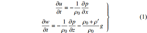
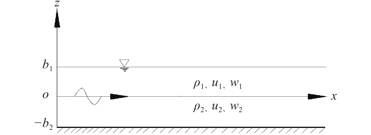
小振幅内波问题可归结为二维的线性问题。假定海水中没有其他流动,x轴取在静止的两层流体交界面上,z轴取向上为正,如图1所示,则不可压缩流体的运动方程和连续性方程可表示为[11]:
![]() 图 1 稳定层化两层流体中内波传播示意Figure 1. Sketch of propagation of internal waves in density stratified two-layer fluid
图 1 稳定层化两层流体中内波传播示意Figure 1. Sketch of propagation of internal waves in density stratified two-layer fluid$$ \left. {\begin{array}{*{20}{c}} {\dfrac{{\partial u}}{{\partial t}} = - \dfrac{1}{{{\rho _0}}}\dfrac{{\partial p}}{{\partial x}}} \\ {\dfrac{{\partial w}}{{\partial t}} = - \dfrac{1}{{{\rho _0}}}\dfrac{{\partial p}}{{\partial {\textit{z}}}} - \dfrac{{{\rho _0} + \rho '}}{{{\rho _0}}}g} \end{array}} \right\} $$ (1) $$ \frac{{\partial u}}{{\partial x}} + \frac{{\partial w}}{{\partial {\textit{z}}}} = 0 $$ (2) 式中:
$ u $ 和$ w $ 分别为流体质点水平和垂向速度;$ t $ 为时间;$ p $ 为压强;$\; {\rho _0} = {\rho _0}({\textit{z}})$ 为静止时分层流体稳定的密度分布,假定其只随深度变化;$\; \rho ' $ 为流体的扰动密度;g为重力加速度。假定上、下层流体交界面处内波频率为
$ \omega $ 、水平波数为$ k $ ,文献[11]推导了刚盖假定下内波的频散关系式和速度场理论解;文献[12-14]推导了自由表面边界条件下内波的频散关系式和速度场理论解。刚盖假定下的频散关系式为:$$ {\omega ^2} = \frac{{({\rho _2} - {\rho _1})gk{\rm{sh}}(k{b_1)}{\rm{sh}}(k{b_2)}}}{{{\rho _1}{\rm{ch}}(k{b_1)}{\rm{sh}}(k{b_2)} + {\rho _2}{\rm{ch}}(k{b_2)}{\rm{sh}}(k{b_1)}}} $$ (3) 式中:
$\;{\rho _{\text{1}}}$ 、$\;{\rho _{\text{2}}}$ 分别为上、下层流体密度;${b_1}$ 、${b_2}$ 分别为上、下层流体深度。自由表面假定下的频散关系式为:
$$ {\left( {\frac{k}{{{k_0}}}} \right)^2}(1 - \gamma ){t_1}{t_2} - \frac{k}{{{k_0}}}({t_1} + {t_2}) + \gamma {t_1}{t_2} + 1 = 0 $$ (4) 式中:
$ {k_0} = {\omega ^2}/g $ ;$ \gamma = {\rho _1}/{\rho _2} $ ;${t_1} = {\rm{th}}(k{b_1})$ ,${t_2} = {\rm{th}}(k{b_2})$ 。2. 两层流体中内波传播的数值模型
2.1 模型的建立及边界条件的设置
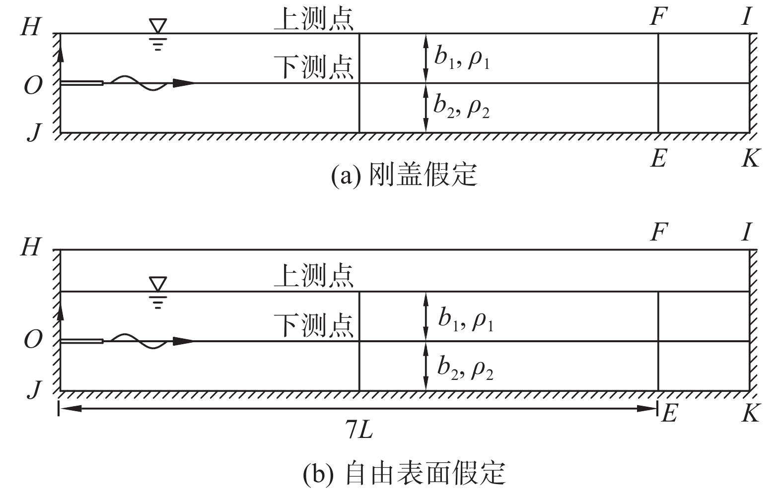
数值水槽如图2所示,原点取在模型左侧的两层流体交界处。数值水槽中内波传播的有效区域为HJEF,其长度取各工况下7倍波长L,消波区域为FEKI,消波区长度取为1.5L,设定总水深为100 m。给定振幅A为1.0 m,周期T为400 s。
本文采用FLUENT软件中的
$k{\text{-}}\varepsilon$ 模型进行数值模拟,并利用VOF(Volume Of Fluid)方法追踪自由液面位置,模型的控制方程和VOF法的介绍可参见文献[6, 15],方程的离散采用了有限体积法。通过改变HI处的边界条件来实现两种边界条件下内波传播的数值模拟。在模拟刚盖假定下内波的传播时,HI处为对称(symmetry)边界条件;模拟自由表面假定下内波的传播时,增加高度为50 m的空气层,空气层上表面HI处为压力进口(Pressure inlet)边界条件。设HJ、JK和KI均为固壁边界条件。模型采用结构化网格,传播区x方向网格大小为各工况波长L的2%;在两层流体交界面以及上层流体的上表面及其邻近处,z方向采用加密网格,其余位置z方向网格均取1 m。在消波区域的
$ x $ 方向采用1.05倍网格大小递增的渐变网格。控制流场全局库朗数(Courant number)为0.02,让FLUENT自动选择合适的时间步长,总模拟时间为6 000 s。2.2 数值造波与消波
采用平板拍击的方法来实现造波[16]。造波板上下拍动,带动流体运动以达到造波的目的,其平衡位置在两层密度不同的流体交界面处。根据体积守恒定律,造波板上下拍击时所排开的流体体积,与波面从造波板边缘沿内波传播方向至无穷远处的积分相等,即:
$$ D{\textit{z}}(t) = \int\limits_D^\infty {\eta (x,t){\text{d}}} x $$ (5) 式中:
$ D $ 为造波板长;$ {\textit{z}}(t) $ 为某时刻造波板偏离平衡位置的距离;$ \eta (x,t) $ 为两层流体交界面处波面位移函数。由于内波沿x轴正向传播,因此:
$$ \frac{{\partial \eta }}{{\partial t}} = - c\frac{{\partial \eta }}{{\partial x}} $$ (6) 式中:
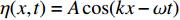
$c$ 为内波相速度。将式(5)两侧对时间求导,再结合式(6),设$\eta (x,t) = A\cos (kx - \omega t)$ ,推导可得:$$ {u_{\text{m}}}(t) = \frac{{cA}}{D}\cos (kD - wt) $$ (7) 式中:
$ {u_{\text{m}}}(t) $ 为造波板垂向运动速度。由式(7)可见运动函数由需要生成的内波波速、振幅、波数、频率和造波板长度确定。采用FLUENT用户自定义函数(UDF)中的刚体运动DEFINE_CG_MOTION宏,结合推导的运动方程,控制造波板上下平移。
在水槽的末端,即在FEKI区域设置消波层进行消波。消波的方法是在消波区内,在每个迭代步内速度u和w都要乘以消波系数
$ \; \mu (x) $ 。$ \mu (x) $ 有线性和指数等多种形式。现选取线性形式:$$ \mu (x) = a\frac{{x - {x_0}}}{B} $$ (8) 式中:
$ a $ 为常数,本文取为0.02;$ {x_0} $ 为消波区起始位置水平坐标;$ x $ 为消波区内任一点的水平坐标;B为消波区长度,常取为1~2倍波长L。2.3 敏感性分析
为了验证计算结果的正确性,需对采用不同
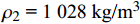
$\Delta {\textit{z}}$ 大小网格的计算结果进行敏感性分析。采用$\;{\rho _{\text{1}}}{\text{ = 1 020 kg/}}{{\text{m}}^3}$ 、$\;{\rho _2}{\text{ = 1 028 kg/}}{{\text{m}}^3}$ 、${b_1} = {\text{10 m}}$ 、${b_2} = $ $ 90{\text{ m}}$ 的刚盖假定数值水槽作为对比分析算例,该算例比其他算例(下文论及)的数值解与相应理论解之间的差别要大。$\Delta {\textit{z}}$ 分别取0.5和1.0 m。图3是$x = $ $ 1{\text{ }}200$ m、${\textit{z}} = 0$ m处流体质点垂向速度随时间的变化曲线。由图3可见,两种网格的计算结果差别很小,与理论解的变化趋势一致。鉴于采用$\Delta {\textit{z}} = {\text{1.0 m}}$ 时能减少计算时间,因此本文采用$\Delta {\textit{z}} = {\text{1.0 m}}$ 的网格进行计算。![]() 图 3 (1 200, 0)处垂向速度随时间的变化过程线Figure 3. Time series of vertical velocity at point (1 200, 0)
图 3 (1 200, 0)处垂向速度随时间的变化过程线Figure 3. Time series of vertical velocity at point (1 200, 0)3. 不同情况下速度场数值解与相应理论解的比较
3.1 上下层流体不同密度差的影响
工况设置如表1所示。假定
$\;{\rho _1}$ 、${\rho _2}$ 、${b_1}$ 、${b_2}$ 四个参数及周期T,用两种假定下的色散关系求得各工况下波数$ k $ (同种工况两种假定下波数$ k $ 均取3位有效数字后近似相等)。由表1可知,在上下层水深及波周期不变的情况下,上下层流体的密度差越大,波数$ k $ 就越小,内波传播速度越快。表 1 上下层不同密度工况设置Table 1. Cases with different densities for upper and lower layers工况 $\;{\rho }_{1}\text{/}(\text{kg}\cdot {\text{m} }^{-3})$ $\;{\rho }_{2}\text{/}(\text{kg}\cdot {\text{m} }^{-3})$ $ {b_1}{\text{/m}} $ $ {b_2}{\text{/m}} $ $ k $ 测点坐标/m Case 1 1 020 1 022 50 50 0.028 7 (750, 0), (750, 50) Case 2 1 020 1 024 50 50 0.018 0 (1 200, 0), (1 200, 50) Case 3 1 020 1 026 50 50 0.014 1 (1 500, 0), (1 500, 50) Case 4 1 020 1 028 50 50 0.012 0 (1 750, 0), (1 750, 50) 在x方向传播区长度的一半处,设置上下两个测点。下测点取在两层流体交界面处(
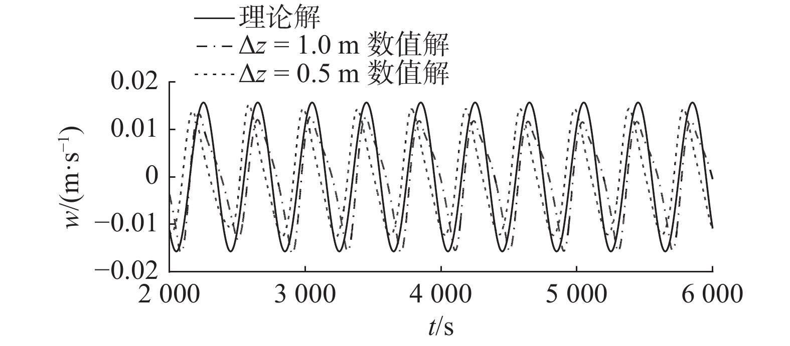
${\textit{z}} = 0$ m),监测该处流体质点的垂向速度$ w $ ;上测点取在上层流体的上表面(${\textit{z}} = 50$ m),监测该处流体质点的垂向速度$ w $ 和水平速度$ u $ 。计算的水气交界面处水平速度结果见图4~5。由于篇幅所限,只给出Case 1及Case 4的部分结果。![]() 图 4 Case 1(750, 50)位置水平速度历时曲线Figure 4. Time series of horizontal velocity at point (750, 50) for Case 1
图 4 Case 1(750, 50)位置水平速度历时曲线Figure 4. Time series of horizontal velocity at point (750, 50) for Case 1![]() 图 5 Case 4(1 750, 50)位置水平速度历时曲线Figure 5. Time series of horizontal velocity at point (1 750, 50) for Case 4
图 5 Case 4(1 750, 50)位置水平速度历时曲线Figure 5. Time series of horizontal velocity at point (1 750, 50) for Case 4由图4~5可知,各工况中的速度在两种边界条件下,数值解与各自的理论解吻合良好;刚盖与自由表面两种边界条件下的数值解基本无差别。对比图4和5可知,如其他条件不变,上下层流体之间密度差越大,上层流体表面的水平速度振幅就越大,水平运动越剧烈。鉴于上层流体表面的垂向速度,在刚盖条件下为0,在自由表面条件下尽管不等于0,但幅值很小,因此没有给出其计算结果图。
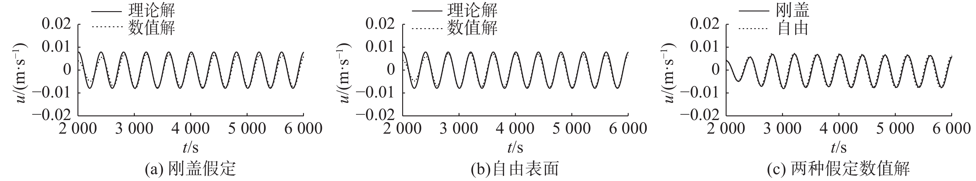
计算了波峰和波谷时垂向速度和水平速度沿水深的分布,波峰和波谷均取在波型充分稳定的时间段。限于篇幅,文中仅给出了水平速度沿水深分布的计算结果,见图6~7。在两种边界条件下,数值解与理论解基本一致。在波峰时刻,下层流体的数值解和理论解吻合得更好;在波谷时刻,上层流体的数值解和理论解吻合得更好。
![]() 图 6 自由表面假定下波峰时水平速度沿水深的分布Figure 6. Distribution of horizontal velocity along water depth at the moment for wave crest under the assumption of free surface
图 6 自由表面假定下波峰时水平速度沿水深的分布Figure 6. Distribution of horizontal velocity along water depth at the moment for wave crest under the assumption of free surface![]() 图 7 刚盖假定下波谷时水平速度沿水深的分布Figure 7. Distribution of horizontal velocity along water depth at the moment for wave trough under the assumption of rigid lid
图 7 刚盖假定下波谷时水平速度沿水深的分布Figure 7. Distribution of horizontal velocity along water depth at the moment for wave trough under the assumption of rigid lid3.2 上下层流体不同水深比的影响
工况设置如表2所示。控制上下层流体的密度不变,改变深度比。由于篇幅所限,只给出工况较为极端的Case 5和Case 8的计算结果,不同位置处流体质点的速度历时曲线见图8~12。
表 2 上下层不同水深工况设置Table 2. Cases with different water depths of upper and lower layers工况 $\; {\rho }_{1}\text{/}(\text{kg}\cdot {\text{m} }^{-3})$ $\; {\rho }_{2}\text{/}(\text{kg}\cdot {\text{m} }^{-3})$ $ {b_1}{\text{/m}} $ $ {b_2}{\text{/m}} $ $ k $ 测点坐标 Case 5 1 020 1 028 10 90 0.019 8 (1 200, 0), (1 200, 10) Case 6 1 020 1 028 20 80 0.014 9 (1 500, 0), (1 500, 20) Case 7 1 020 1 028 80 20 0.014 9 (1 500, 0), (1 500, 80) Case 8 1 020 1 028 90 10 0.019 8 (1 200, 0), (1 200, 90) ![]() 图 8 Case 5(1 200, 0)位置垂向速度历时曲线Figure 8. Time series of vertical velocity at point (1 200, 0) for Case 5
图 8 Case 5(1 200, 0)位置垂向速度历时曲线Figure 8. Time series of vertical velocity at point (1 200, 0) for Case 5![]() 图 9 Case 5(1 200, 10)位置垂向速度数值解历时曲线Figure 9. Time series of numerical vertical velocity at point (1 200, 10) for Case 5
图 9 Case 5(1 200, 10)位置垂向速度数值解历时曲线Figure 9. Time series of numerical vertical velocity at point (1 200, 10) for Case 5![]() 图 10 Case 5(1 200, 10)位置水平速度数值解历时曲线Figure 10. Time series of numerical horizontal velocity at point (1 200, 10) for Case 5
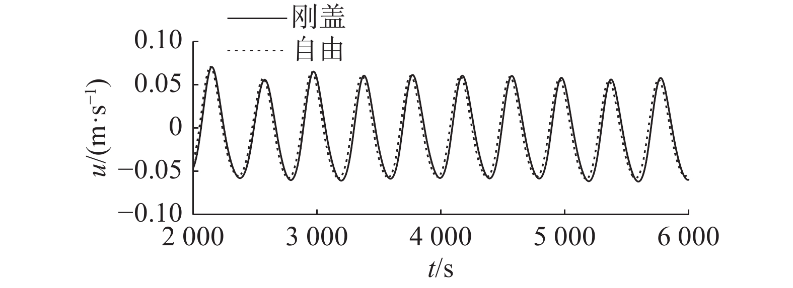
图 10 Case 5(1 200, 10)位置水平速度数值解历时曲线Figure 10. Time series of numerical horizontal velocity at point (1 200, 10) for Case 5![]() 图 11 Case 8(1 200, 0)位置垂向速度历时曲线Figure 11. Time series of vertical velocity at point (1 200, 0) for Case 8
图 11 Case 8(1 200, 0)位置垂向速度历时曲线Figure 11. Time series of vertical velocity at point (1 200, 0) for Case 8由表2可以明显看出,当上下层流体深度
$ {b_1} $ 、$ {b_{\text{2}}} $ 互换时,波数$ k $ 近似相等,这体现了色散方程的“对偶性”[17]。由图8和11可见,两层流体交界面处的垂向速度,无论在哪种边界条件下,数值解与理论解相比均已有较大区别,体现出一定的非线性影响;当
$ {b_1} $ 小于$ {b_{\text{2}}} $ 时,数值解的波峰处幅值小于波谷处幅值;当$ {b_1} $ 大于$ {b_{\text{2}}} $ 时,数值解的波峰处幅值大于波谷处幅值。当$ {b_1} $ 小于$ {b_{\text{2}}} $ 时,刚盖假定下所计算的垂向速度幅值大于自由表面假定下所计算的垂向速度幅值;当$ {b_1} $ 大于$ {b_{\text{2}}} $ 时则相反。由图9可见,当
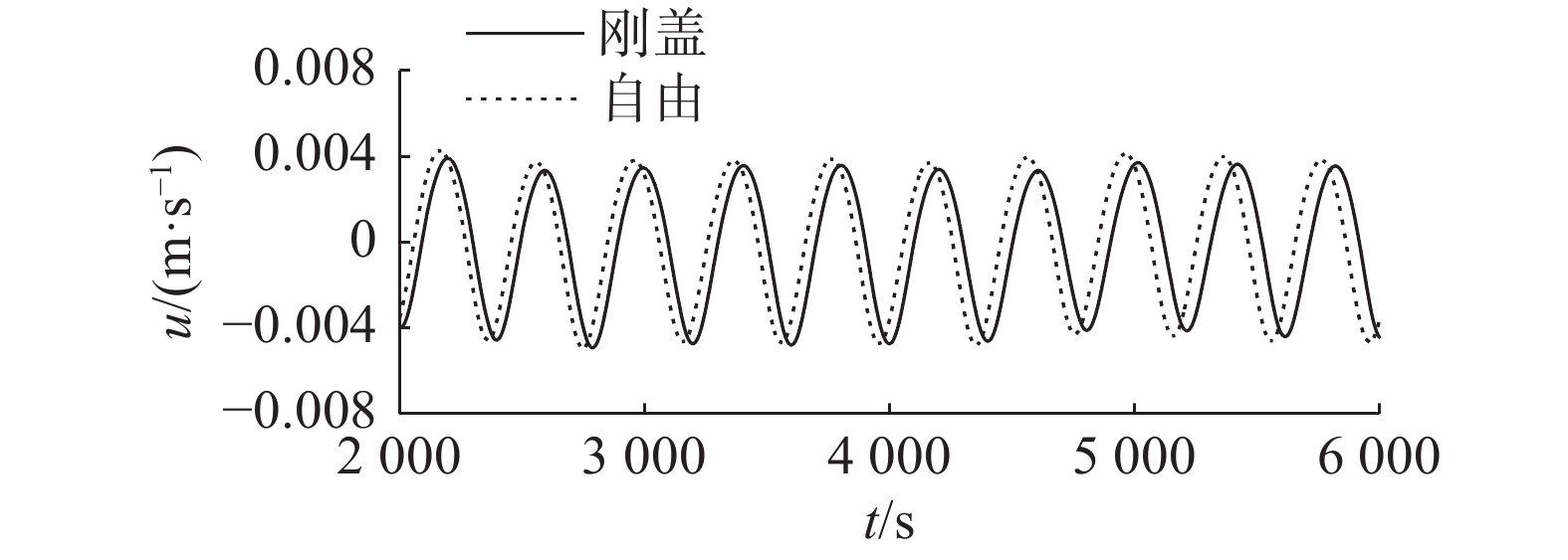
$ {b_1} $ 很小时,自由表面假定下的数值解有明显的波动。而当$ {b_1} $ 大于$ {b_{\text{2}}} $ 时,波动几乎为0,因此文中没有给出其计算结果图。图10和12是上层流体表面的水平速度随时间变化曲线。可见,当$ {b_1} $ 小于$ {b_{\text{2}}} $ 时,数值解的波峰尖陡、波谷平坦,呈现出非线性影响;而当$ {b_1} $ 大于$ {b_{\text{2}}} $ 时,则非线性影响微弱。在入射条件相同的情况下,$ {b_1} $ 越小上层流体的表面速度越大。鉴于波谷时刻与波峰时刻的速度沿水深分布图相类似及两种假定下数值计算结果类似,文中仅给出了波峰时的垂向和水平速度沿水深分布,见图13~14,R代表刚盖,F代表自由表面。由图13可见数值解垂向速度的极大值不再位于两层流体交界面处。
$ {b_1} $ 小于$ {b_{\text{2}}} $ 时,垂向速度极大值的位置向下偏移,导致监测点记录的数据更小;$ {b_1} $ 大于$ {b_{\text{2}}} $ 时,极大值的位置向上偏移,监测点记录到的数据也更小。在图8和11中也体现出波峰时数值解的幅值相对于理论解有所偏小。图14是波峰时刻水平速度沿水深的分布。由图14可见,密跃层越靠近上层表面,上层流体内数值解和理论解差别越大,下层流体内差别越小,反之亦然。同种工况内,两种边界条件下的流体质点水平速度沿水深的分布,没有明显的区别。![]() 图 12 Case 8(1 200, 90)位置水平速度数值解历时曲线Figure 12. Time series of numerical horizontal velocity at point (1 200, 90) for Case 8
图 12 Case 8(1 200, 90)位置水平速度数值解历时曲线Figure 12. Time series of numerical horizontal velocity at point (1 200, 90) for Case 8![]() 图 13 波峰时垂向速度沿水深的分布图Figure 13. Distribution of vertical velocity along water depth at the moment for wave crest
图 13 波峰时垂向速度沿水深的分布图Figure 13. Distribution of vertical velocity along water depth at the moment for wave crest![]() 图 14 波峰时水平速度沿水深的分布图Figure 14. Distribution of horizontal velocity along water depth at the moment for wave crest
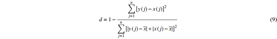
图 14 波峰时水平速度沿水深的分布图Figure 14. Distribution of horizontal velocity along water depth at the moment for wave crest各工况在波峰波谷时刻,水平速度与垂向速度的数值解和理论解之间的一致程度可用指标d来衡量[18-19]:
$$ d = 1 - \frac{{\displaystyle\sum\limits_{j = 1}^n {{{\left[ {y\left( j \right) - x\left( j \right)} \right]}^2}} }}{{\displaystyle\sum\limits_{j = 1}^n {{{\left[ {\left| {y\left( j \right) - \overline x } \right| + \left| {x\left( j \right) - \overline x } \right|} \right]}^2}} }} $$ (9) 式中:
$x\left( j \right)$ 为理论解;$\overline x $ 为理论解均值;$y\left( j \right)$ 为数值解。$d = 0$ 时表示数值解与理论解完全不一致,而$d = 1$ 表示数值解与理论解完美匹配。由表3及图4~7可见,Case 1~Case 4尽管下层流体密度不同,但上下两层深度相等,密跃层刚好位于水深的1/2处,此时总体说来,数值解与理论解相差较小。Case 5~Case 8上下两层流体密度固定,但上下两层深度差别较大,由表3及图8~14可见,此时数值解与理论解的差别较大。特别是当上下两层水深差值较大时,数值解与理论解的差别更大,其中又以密跃层接近静水面时表现得更为明显,这体现了非线性的影响。这是因为数值解是非线性解,而理论解是线性解。在上层水深很小时,在自由表面假定下水气交界面处出现了较为明显的垂向速度。鉴于在实际海洋中上层水深远小于下层水深,由此可以推断,对于实际的海洋分层流体,采用更为真实的自由表面假定应更为合理。
表 3 各工况水平和垂向速度的数值解和理论解一致性分析Table 3. Consistency analysis between the numerical and analytical results for the horizontal and vertical velocities of different casesd Case 1 Case 2 Case 3 Case 4 Case 5 Case 6 Case 7 Case 8 $ d{\left(w峰\right)}_{\text{R}} $ 0.999 8 0.999 8 0.998 7 0.997 3 0.938 9 0.988 4 0.993 2 0.994 2 $ d{\left(w峰\right)}_{\text{F}} $ 0.996 4 0.996 0 0.998 9 0.998 2 0.927 5 0.984 2 0.997 0 0.996 6 $ d{\left(u峰\right)}_{\text{R}} $ 0.992 2 0.994 4 0.997 1 0.997 6 0.971 1 0.995 4 0.992 5 0.968 3 $ d{\left(u峰\right)}_{\text{F}} $ 0.994 1 0.996 0 0.997 1 0.997 0 0.962 8 0.996 2 0.994 4 0.979 8 $ d{\left(w谷\right)}_{\text{R}} $ 0.999 8 0.999 8 0.998 5 0.999 8 0.993 4 0.995 2 0.994 2 0.977 7 $ d{\left(w谷\right)}_{\text{F}} $ 0.994 7 0.995 9 0.997 3 0.998 9 0.979 0 0.997 4 0.992 5 0.978 0 $ d{\left(u谷\right)}_{\text{R}} $ 0.993 8 0.995 5 0.997 8 0.998 2 0.977 4 0.996 0 0.996 8 0.972 6 $ d{\left(u谷\right)}_{\text{F}} $ 0.995 1 0.997 1 0.998 0 0.998 3 0.971 3 0.995 8 0.996 8 0.987 5 注:R代表刚盖,F代表自由表面。 4. 结 语
本文基于
$k{\text{-}}\varepsilon$ 模型和VOF方法,以FLUENT软件为计算平台,采用平板造波的方法,实现了刚盖假定和自由表面假定下小振幅内波传播的数值模拟,通过比较z方向不同网格大小的计算结果,检验了计算结果的合理性。设置上下两层流体不同的密度差和深度,数值模拟了刚盖假定和自由表面假定下多种情况内波的传播;通过与各自理论解的比较,阐述了数值解与理论解之间的异同;通过对两种假定下计算结果的比较,分析了两种假定下数值计算结果之间的差别及其产生的原因。在上下层水深相同的前提下,尽管上下层流体密度差不同,但此时总体上数值解与理论解相吻合;尽管在自由表面假定下,静水面处存在垂向速度,但其数值很小。在上下两层流体密度差固定的前提下,上下两层流体深度差值的改变会较为明显地影响数值计算结果,以密跃层接近海洋上表面时表现得更为明显,此时数值解与理论解差别较大,这体现了非线性的影响;在自由表面假定下出现了较为明显的垂向速度,这体现了海洋上表面边界条件的影响;在给定入射条件下,上层流体水深越小,上表面处速度越大。
鉴于在实际海洋中,一般密跃层以上水深远小于下层水深。当计算运动幅值更大的内孤立波时,可以设想此时边界条件的影响会更加明显,这便是本研究意义所在,也是下一步将要研究的内容。本文工作也为内波与表面波之间相互作用的研究提供了参考。
-
![]()
图 1 稳定层化两层流体中内波传播示意
Figure 1. Sketch of propagation of internal waves in density stratified two-layer fluid
![]()
图 3 (1 200, 0)处垂向速度随时间的变化过程线
Figure 3. Time series of vertical velocity at point (1 200, 0)
![]()
图 4 Case 1(750, 50)位置水平速度历时曲线
Figure 4. Time series of horizontal velocity at point (750, 50) for Case 1
![]()
图 5 Case 4(1 750, 50)位置水平速度历时曲线
Figure 5. Time series of horizontal velocity at point (1 750, 50) for Case 4
![]()
图 6 自由表面假定下波峰时水平速度沿水深的分布
Figure 6. Distribution of horizontal velocity along water depth at the moment for wave crest under the assumption of free surface
![]()
图 7 刚盖假定下波谷时水平速度沿水深的分布
Figure 7. Distribution of horizontal velocity along water depth at the moment for wave trough under the assumption of rigid lid
![]()
图 8 Case 5(1 200, 0)位置垂向速度历时曲线
Figure 8. Time series of vertical velocity at point (1 200, 0) for Case 5
![]()
图 9 Case 5(1 200, 10)位置垂向速度数值解历时曲线
Figure 9. Time series of numerical vertical velocity at point (1 200, 10) for Case 5
![]()
图 10 Case 5(1 200, 10)位置水平速度数值解历时曲线
Figure 10. Time series of numerical horizontal velocity at point (1 200, 10) for Case 5
![]()
图 11 Case 8(1 200, 0)位置垂向速度历时曲线
Figure 11. Time series of vertical velocity at point (1 200, 0) for Case 8
![]()
图 12 Case 8(1 200, 90)位置水平速度数值解历时曲线
Figure 12. Time series of numerical horizontal velocity at point (1 200, 90) for Case 8
![]()
图 13 波峰时垂向速度沿水深的分布图
Figure 13. Distribution of vertical velocity along water depth at the moment for wave crest
![]()
图 14 波峰时水平速度沿水深的分布图
Figure 14. Distribution of horizontal velocity along water depth at the moment for wave crest
表 1 上下层不同密度工况设置
Table 1 Cases with different densities for upper and lower layers
工况 $\;{\rho }_{1}\text{/}(\text{kg}\cdot {\text{m} }^{-3})$ $\;{\rho }_{2}\text{/}(\text{kg}\cdot {\text{m} }^{-3})$ $ {b_1}{\text{/m}} $ $ {b_2}{\text{/m}} $ $ k $ 测点坐标/m Case 1 1 020 1 022 50 50 0.028 7 (750, 0), (750, 50) Case 2 1 020 1 024 50 50 0.018 0 (1 200, 0), (1 200, 50) Case 3 1 020 1 026 50 50 0.014 1 (1 500, 0), (1 500, 50) Case 4 1 020 1 028 50 50 0.012 0 (1 750, 0), (1 750, 50)  下载: 导出CSV
表 2 上下层不同水深工况设置
Table 2 Cases with different water depths of upper and lower layers
工况 $\; {\rho }_{1}\text{/}(\text{kg}\cdot {\text{m} }^{-3})$ $\; {\rho }_{2}\text{/}(\text{kg}\cdot {\text{m} }^{-3})$ $ {b_1}{\text{/m}} $ $ {b_2}{\text{/m}} $ $ k $ 测点坐标 Case 5 1 020 1 028 10 90 0.019 8 (1 200, 0), (1 200, 10) Case 6 1 020 1 028 20 80 0.014 9 (1 500, 0), (1 500, 20) Case 7 1 020 1 028 80 20 0.014 9 (1 500, 0), (1 500, 80) Case 8 1 020 1 028 90 10 0.019 8 (1 200, 0), (1 200, 90)
下载: 导出CSV
表 3 各工况水平和垂向速度的数值解和理论解一致性分析
Table 3 Consistency analysis between the numerical and analytical results for the horizontal and vertical velocities of different cases
d Case 1 Case 2 Case 3 Case 4 Case 5 Case 6 Case 7 Case 8 $ d{\left(w峰\right)}_{\text{R}} $ 0.999 8 0.999 8 0.998 7 0.997 3 0.938 9 0.988 4 0.993 2 0.994 2 $ d{\left(w峰\right)}_{\text{F}} $ 0.996 4 0.996 0 0.998 9 0.998 2 0.927 5 0.984 2 0.997 0 0.996 6 $ d{\left(u峰\right)}_{\text{R}} $ 0.992 2 0.994 4 0.997 1 0.997 6 0.971 1 0.995 4 0.992 5 0.968 3 $ d{\left(u峰\right)}_{\text{F}} $ 0.994 1 0.996 0 0.997 1 0.997 0 0.962 8 0.996 2 0.994 4 0.979 8 $ d{\left(w谷\right)}_{\text{R}} $ 0.999 8 0.999 8 0.998 5 0.999 8 0.993 4 0.995 2 0.994 2 0.977 7 $ d{\left(w谷\right)}_{\text{F}} $ 0.994 7 0.995 9 0.997 3 0.998 9 0.979 0 0.997 4 0.992 5 0.978 0 $ d{\left(u谷\right)}_{\text{R}} $ 0.993 8 0.995 5 0.997 8 0.998 2 0.977 4 0.996 0 0.996 8 0.972 6 $ d{\left(u谷\right)}_{\text{F}} $ 0.995 1 0.997 1 0.998 0 0.998 3 0.971 3 0.995 8 0.996 8 0.987 5 注:R代表刚盖,F代表自由表面。
下载: 导出CSV
-
[1] 张洪生, 郑应刚, 王有强. 基于VMD对SAR海洋内波参数的自动反演[J]. 海洋工程,2021,39(3):1-10. (ZHANG Hongsheng, ZHENG Yinggang, WANG Youqiang. Automatically extracting parameters of oceanic internal wave from SAR image based on variational mode decomposition[J]. The Ocean Engineering, 2021, 39(3): 1-10. (in Chinese) [2] 王火平, 陈亮, 郭延良, 等. 海洋内孤立波预警监测识别技术及其在流花16-2油田群开发中的应用[J]. 海洋工程,2021,39(2):162-170. (WANG Huoping, CHEN Liang, GUO Yanliang, et al. Observing, identification and early warning technology of internal solitary wave and its application in Liuhua 16-2 oilfield group development project[J]. The Ocean Engineering, 2021, 39(2): 162-170. (in Chinese) [3] ZHANG H S, JIA H Q, GU J B, et al. Numerical simulation of the internal wave propagation in continuously density-stratified ocean[J]. Journal of Hydrodynamics, 2014, 26(5): 770-779. doi: 10.1016/S1001-6058(14)60086-X
[4] 李景远, 张庆河, 陈同庆. 密度连续变化水体内孤立波数值模拟研究[J]. 天津大学学报(自然科学与工程技术版),2021,54(2):161-170. (LI Jingyuan, ZHANG Qinghe, CHEN Tongqing. Numerical simulation of internal solitary wave in continuously stratified fluid[J]. Journal of Tianjin University (Science and Technology), 2021, 54(2): 161-170. (in Chinese) [5] 高原雪, 尤云祥, 王旭, 等. 基于MCC理论的内孤立波数值模拟[J]. 海洋工程,2012,30(4):29-36. (GAO Yuanxue, YOU Yunxiang, WANG Xu, et al. Numerical simulation for the internal solitary wave based on MCC theory[J]. The Ocean Engineering, 2012, 30(4): 29-36. (in Chinese) [6] 陈钰, 朱良生. 基于FLUENT的海洋内孤立波数值水槽模拟[J]. 海洋技术,2009,28(4):72-75, 100. (CHEN Yu, ZHU Liangsheng. Numerical wave tank simulation of oceanic internal solitary waves based on FLUENT[J]. Ocean Technology, 2009, 28(4): 72-75, 100. (in Chinese) doi: 10.3969/j.issn.1003-2029.2009.04.021 [7] TEREZ D E, KNIO O M. Numerical simulations of large-amplitude internal solitary waves[J]. Journal of Fluid Mechanics, 1998, 362: 53-82. doi: 10.1017/S0022112098008799
[8] 韩鹏, 钱洪宝, 李宇航, 等. 内波的生成、传播、遥感观测及其与海洋结构物相互作用研究进展[J]. 海洋工程,2020,38(4):148-158. (HAN Peng, QIAN Hongbao, LI Yuhang, et al. Generation, propagation and detection of internal wave and its interaction with ocean structures[J]. The Ocean Engineering, 2020, 38(4): 148-158. (in Chinese) [9] BAIE M A, PIROOZNIA M, AKBARINASAB M. Simulation of the internal wave of a subsurface vehicle in a two-layer stratified fluid[J]. Journal of Ocean University of China, 2020, 19(6): 1255-1264. doi: 10.1007/s11802-020-4223-9
[10] 刘亚男, 郭晓宇, 王本龙, 等. 基于RANS方程的海堤越浪数值模拟[J]. 水动力学研究与进展(A辑),2007,22(6):682-688. (LIU Yanan, GUO Xiaoyu, WANG Benlong, et al. Numerical simulation of wave overtopping over seawalls using the RANS equations[J]. Journal of Hydrodynamics (SerA), 2007, 22(6): 682-688. (in Chinese) [11] 叶安乐, 李凤岐. 物理海洋学[M]. 青岛: 青岛海洋大学出版社, 1992. YE Anle, LI Fengqi. Physical oceanography[M]. Qingdao: Qingdao Ocean University Press, 1992. (in Chinese)
[12] 方欣华, 杜涛. 海洋内波基础和中国海内波[M]. 青岛: 中国海洋大学出版社, 2005. FANG Xinhua, DU Tao. Fundamentals of oceanic internal waves and internal waves in the China seas[M]. Qingdao: China Ocean University Press, 2005. (in Chinese)
[13] 文圣常, 余宙文. 海浪理论与计算原理[M]. 北京: 科学出版社, 1984. WEN Shengchang, YU Zhouwen. Wave theory and its calculation principle[M]. Beijing: Science Press, 1984. (in Chinese)
[14] YEUNG R W, NGUYEN T C. Waves generated by a moving source in a two-layer ocean of finite depth[J]. Journal of Engineering Mathematics, 1999, 35(1): 85-107.
[15] 邓成进, 袁秋霜, 侯延华, 等. 基于FLUENT的库区涌浪数值模拟[J]. 水利水运工程学报,2014(3):84-91. (DENG Chengjin, YUAN Qiushuang, HOU Yanhua, et al. Numerical simulation of the surge based on FLUENT software[J]. Hydro-Science and Engineering, 2014(3): 84-91. (in Chinese) doi: 10.3969/j.issn.1009-640X.2014.03.013 [16] 徐鑫哲. 内波生成机理及二维内波数值水槽模型研究[D]. 哈尔滨: 哈尔滨工程大学, 2012. XU Xinzhe. Study on generational mechanism and 2-D numerical flume model of internal waves[D]. Harbin: Harbin Engineering University. (in Chinese)
[17] 姜胜超, 滕斌, 勾莹. 两种水面边界条件下的内波解及其比较[J]. 中国海洋平台,2008,23(3):11-16. (JIANG Shengchao, TENG Bin, GOU Ying. The characters and comparison of two internal wave solutions with different surface conditions[J]. China Offshore Platform, 2008, 23(3): 11-16. (in Chinese) doi: 10.3969/j.issn.1001-4500.2008.03.002 [18] WILLMOTT C J. On the validation of models[J]. Physical Geography, 1981, 2(2): 184-194. doi: 10.1080/02723646.1981.10642213
[19] ZHANG H S, ZHU L S, YOU Y X. A numerical model for wave propagation in curvilinear coordinates[J]. Coastal Engineering, 2005, 52(6): 513-533. doi: 10.1016/j.coastaleng.2005.02.004
-
期刊类型引用(1)
1. 姚宇,常海超,闫晓青. 三峡升船机成组船舶进厢水动力性能研究. 武汉理工大学学报. 2024(02): 88-93 .  百度学术
百度学术
其他类型引用(0)


计量
- 文章访问数: 330
- HTML全文浏览量: 324
- PDF下载量: 35
- 被引次数: 1
